New Gooroo waiting times formula
09/08/2013by Rob Findlay
At 4.30pm on Friday 30th August we will implement implemented a new formula to improve the waiting times calculations throughout our software. This post explains why the change is being made and the effect it will have.
In summary: The new formula is much better at handling small waiting lists and times. The old formula sometimes gave unduly short (or even negative) waiting times in some circumstances, and the new formula fixes this. As a consequence the new formula often returns slightly higher waiting times at larger list sizes, particularly for flux-based waiting times targets (i.e. those that measure waits as the patients come in, for example admitted patient waiting times). The exact difference varies according to the characteristics of the waiting list but is of the order of one week.
We know that users of Gooroo software base their plans on our waiting time calculations, so changing the waiting times formula is not a step that we take lightly. We hope that by making the change during the summer holidays, and before the annual planning round begins in earnest, we have minimised any possible disruption. We are of course ready to answer any questions and support you if you have any issues around this change: email support@gooroo.co.uk
What changes will I notice in Gooroo Planner?
The waiting times calculated in Gooroo Planner will be slightly different after the new formula is introduced. Also, if you create a report using the activity scenario “Match waiting list targets” then the calculated activity, capacity and list size will be slightly different; if you want to preserve the existing activity levels, a new facility will be released at the time of the change (is has been: you’ll find a new “Convert to dataset” icon in the Report Manager) to allow you to convert your pre-existing waiting-time-driven reports into activity-driven datasets with the activity levels unaltered.
The waiting times formula is only applied when the calculations are actually run. Obviously the calculations are run for all services when you create a brand new report from any dataset. They are also run every time you run Profiling, so for older reports you will find that the waiting time profiles generated on-screen do not finish the future period at the same waiting time that is shown in the main Report table. The calculations are also run when you edit an individual service in an existing report, and in this case the calculations are re-run for that service and others closely related to it (i.e. where all headers match apart from HeadType).
But if you have already created a report, and do not edit it, then all the numbers in the main report table will remain unchanged. So there is no need to download snapshots of existing reports just to preserve a record of them.
Why change the formula?
The old waiting times formula was developed from intensive simulation research into the patient booking process, covering over a billion simulated bookings in all. As far as we know, it was the first time that waiting times had been determined in this way, taking into account factors like removals from the waiting list, full or partial booking, and “x% within y weeks” targets, as well as factors such as the list size, addition rate, and clinical urgency (which I had previously linked to waiting times on a theoretical basis in the mid-1990s).
The original research assumed, logically, that routine waits are significantly longer than urgent waits, and so it focussed on routine waiting times of several weeks which was consistent with typical waits in the NHS at the time. However as Gooroo has become more widely used around the NHS, and as waiting times have continued to fall, we have found that people are increasingly modelling quite short waiting lists and times; we noticed that our old waiting times formula sometimes gave results that were too short (and in some circumstances negative) when applied to very small waiting lists, and this was starting to matter.
We therefore needed to revise our formula to handle short waiting times better, and in particular to avoid giving negative results. If there are zero patients on the waiting list, then the waiting time (however defined) should be zero. The new formula achieves this, and is based on new simulation research that covers a wider range of scenarios and studied over 50 million additional simulated patient bookings.
Comparison of old and new formulae
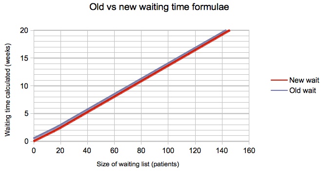
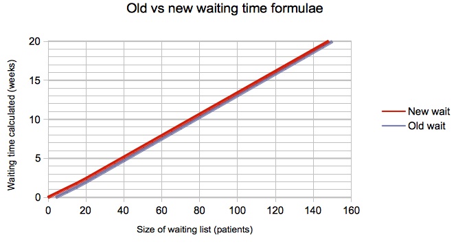
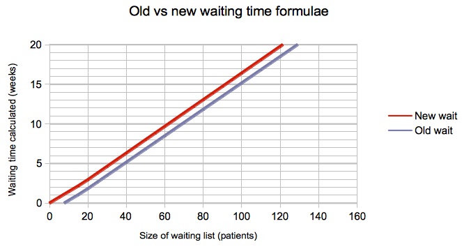
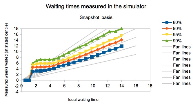
The results given by the old and new formulae are compared in the next few charts, for one of the scenarios we researched where 25% of patients are clinically urgent and 15% of patients are removed from the waiting list for reasons other than treatment.
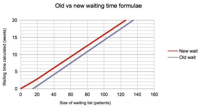
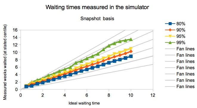
You can see that there is negligible change in the snapshot-based waits below (which converged close to zero already), and an increase of just over a week for flux-based targets, where waits are monitored as the patients are treated (when the old formula gave negative waits for small lists).
The most extreme difference found was for a zero list size with zero urgent patients, zero removals, and partial booking, for which the new formula sensibly returned a zero week wait and the old formula returned a negative wait of -4.5 weeks; however this is not of course a scenario you are ever likely to want to model.
How was the new formula determined?
The first step was to narrow down the factors that need to be taken into account when calculating waiting times. This was covered in our earlier research, and fully written-up in our Research White Paper 5 (see our Publications section).
The second step was to test whether waiting times can be assumed to vary linearly with the ‘ideal’ waiting time, and whether waits and list sizes converge on zero together. (The ‘ideal’ waiting time is the time that all routine patients would wait if there were clinically urgent patients being treated quickly, but there was no randomness or other disruption whatsoever; it is a useful benchmark and modelling concept, though not achievable as a practical objective.)
The chart below shows that the relationship is indeed linear at longer waiting times. At shorter waits, the complicating factor is urgent patients. If, for instance, urgent patients must be treated within 4 weeks, then what happens to them when the list is small and routine waits are only a week or two? If you simulate this naïvely, you end up with results like the chart below, where waiting times “take off” for very small waiting lists, because urgent patients are being kept waiting by the continued enforcement of rules that should no longer apply.
In real life it would make no sense to keep urgent patients waiting up to 4 weeks if routine patients only wait 2 weeks. So in our modelling we have assumed that, as routine waits fall, only the most urgent patients are booked in earlier. As a result the number of patients being managed as “urgent” naturally dwindles as routine waits fall towards zero. Because this is a continuous process, waits continue to fall approximately linearly with the ideal waiting time. As a cross-check, the chart below shows that waiting times also fall linearly (and along similar paths) in the end case of zero urgents.
At the end of these first two steps, then, we had determined that “waiting time divided by ideal wait” is a function of:
- whether the waiting time target is snapshot-based (like incomplete pathways) or flux based (like admitted patients);
- the proportion of patients who must be treated/seen within the target (e.g. 90% for admitted patients);
- whether patients are scheduled under a fully-booked or partially-booked system;
- the proportion of patients removed from the list during their wait.
The ideal wait, in its turn, takes account of the other critical factors such as clinical urgency, the size of waiting list, and the addition rate.
We ran our patient scheduling simulator under a range of scenarios for all those measures, and at different list sizes to cross-check invariance for different ideal waits. For target proportions below 95%, wait-divided-by-ideal was an approximately linear function of the target proportion and the removal rate. For target proportions above 95% it became nonlinear and this was approximated using a different (but still linear) function as shown below.
An example of the fit between the simulator results and the new waiting times function is shown in the following chart, for snapshot-based targets in a fully-booked service, where the vertical axis shows wait-divided-by-ideal, the horizontal axis shows the target proportion, each group of coloured lines from bottom to top shows different removal rates (0%, 5%, 10%, 15%, 20% and 25%), the solid and long-dashed lines show the results from smaller and larger list sizes respectively, the fine-dashed line shows the results of the new waiting times function, and the left and right segments show the different formulae for target proportions below and above 95%.
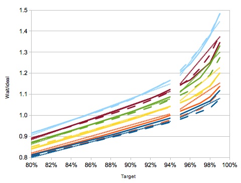
Charts like the one above were generated for all the scenarios studied, to take into account all the factors that significantly affect waiting times. The result was a set of formulae that were calibrated for each scenario and which converged well to zero. This is the new formula set that is being implemented.
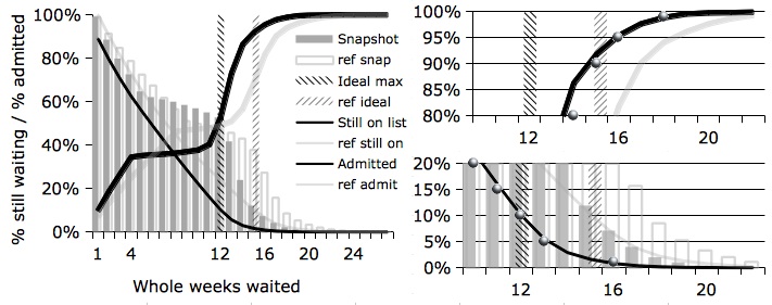
As a final check, the formula was compared against the outputs from the simulator using the same chart format as in our original Research White Paper 5, to make sure that the formula results (silver balls) lie close to the measured performance of the simulator (black lines). The following example is taken from a list size of 90 with 15% removals and a fully-booked service and (like other scenarios) shows a good fit.
Return to Post Index