Calculating bed occupancy and risk – week by week variation

Calculating bed occupancy and risk – week by week variation

30/01/2019
by Rob Findlay

In the previous article we saw that running out of beds has consequences for patients and the hospital. The acceptable risk of that happening, rather than bed occupancy, should be the basis for informed discussions of bed capacity. So when the acceptable level of risk has been agreed, we then need a way of converting it into bed occupancy for capacity planning purposes.

There are several ways of doing this.

We could run a computer simulation, which was how the well-known 85 per cent bed occupancy figure was obtained, taking care to make sure that the distribution of admissions and discharges is realistic.

Or we could use the queueing theory techniques developed by Erlang.

Or we could analyse the variations in non-elective admissions and discharges over different timescales, using real data from the specific beds concerned. This is the method we are going to use here.

The number of non-elective admissions varies a lot from week to week, and also during the week. We’ll look at the week by week variation in this article, and variation during the week in the next.

Predictable or unpredictable

Before we dive into the numbers, we need to think about what bed occupancy is for. It isn’t simply about absorbing variation – it’s about absorbing that variation which we cannot predict and manage by other means. So we know that respiratory admissions rise in winter, and trauma in summer, but we can manage that by adjusting the number of staffed beds and reprofiling elective admissions. Bed occupancy only needs to be low enough to absorb the other variation that we cannot predict and manage.

We therefore need a way of forecasting non-elective admissions, and then we need to test it against some real data to see how well it does. The variation it successfully predicts – with enough notice that we can take action to deal with it – is something we can manage by other means. Whereas any error in those predictions is something we cannot predict and manage, and that is what bed occupancy needs to absorb.

Therefore if we can improve our forecasting, so that less of the variation is unpredictable, then we can operate at higher bed occupancy with fewer beds and lower costs – a nice example of the benefits of good analysis.

How shall we do our forecast? Forecasting is a huge subject, but for current purposes a straightforward approach will suffice. Operational managers often forecast non-elective demand by calculating the average over the last six weeks (considering each weekday separately), and this method performs reasonably well. A slightly more advanced technique is simple exponential smoothing which can be tuned to fit the variability of the data and is fairly easy to do in a spreadsheet; this is the method we will use here because (as we will see in part 6) we need to be sensitive to the patterns of demand in different bed pools.

Week by week variation

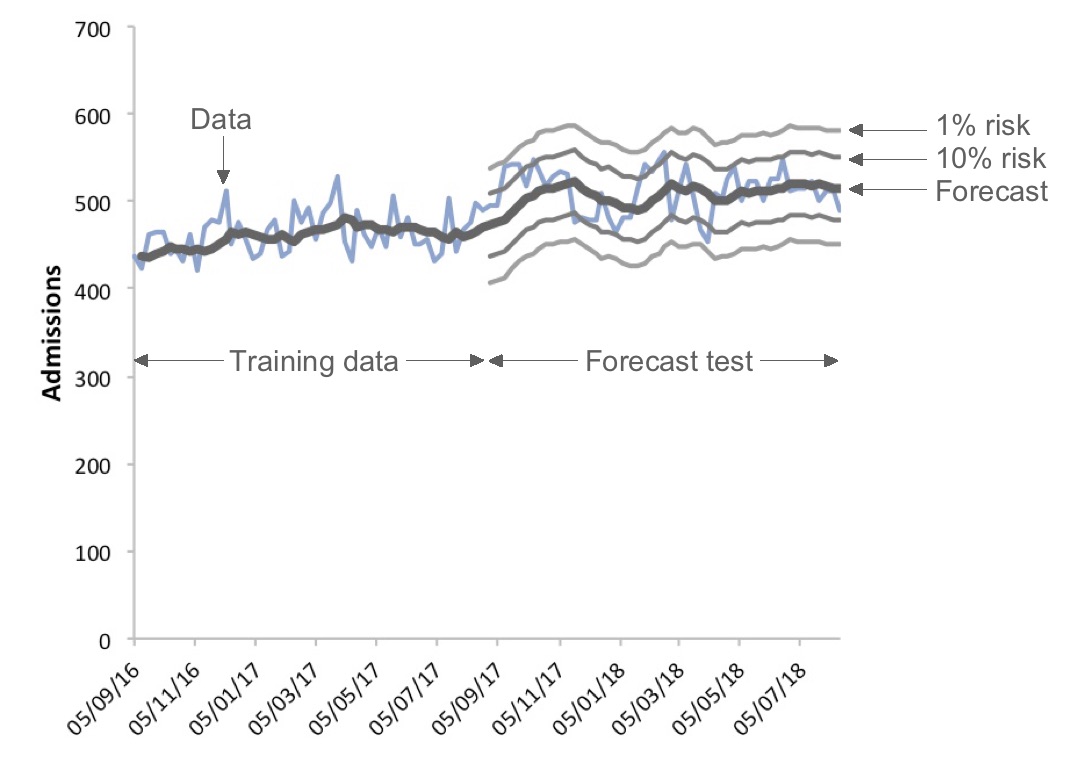
Let’s try it with some real data. The jagged blue line in the chart below shows the actual number of non-elective admissions to adult general and acute beds, in a particular hospital, every week for two years. The first year of data was used to tune the forecasting model, and then the model was allowed to run on through the second year to see how well it performed. Each forecast was just for the following week, and the forecasts are shown by the dark grey line running through the middle.

The other grey lines show how well the forecast performed in the second year. There is a 1 per cent risk of admissions breaching the top grey line in any given week, and a 10 per cent risk of breaching the second grey line down.

Now we are ready to calculate bed occupancy.

If we make enough beds available to cope with the top grey line, then we can expect to run out of beds only 1 per cent of the time. The central forecast line shows the average number of beds that will be occupied. So far, so good.

Now recall that, when planning bed capacity, the bed occupancy is the average proportion of available beds that are occupied over time. Therefore the bed occupancy that is consistent with a 1 per cent risk of running out of beds, is the ratio between the forecast line and the top grey line. And we can use the same method to calculate bed occupancy for any level of risk in this bed pool – which is the result we wanted.

This calculation of bed occupancy takes account of the week-by-week variations in demand, but that is not the complete picture. There are also important variations during the week that need to be taken into account, because of the way that admissions and discharges vary by time of day, and day of week. And that is the subject of the next article in this series.

I would like to thank the Emergency Care Intensive Support Team at NHS Improvement for their helpful suggestions during the preparation of these articles, Piotr Fryzlewicz, Professor of Statistics at the London School of Economics, for reviewing and advising on the statistical methods used, and those acute hospitals in England and Scotland who helped to pilot the methods.

We can calculate the relationship between bed occupancy and risk for your acute hospital – please get in touch if you are interested.

Return to Post Index